As a college algebra teacher, I was not satisfied with the way I presented the intermediate value theorem last trimester. I felt the lesson was somewhat isolated from other concepts we had studied and definitely was disconnected from the real world. My approach lacked a hook and was laddened with procedure. Committed to teaching the concept better this trimester, I recorded the following video while (someone else) was driving:
I know, not a high quality masterpiece, but I think I captured what I needed to illustrate the theorem.
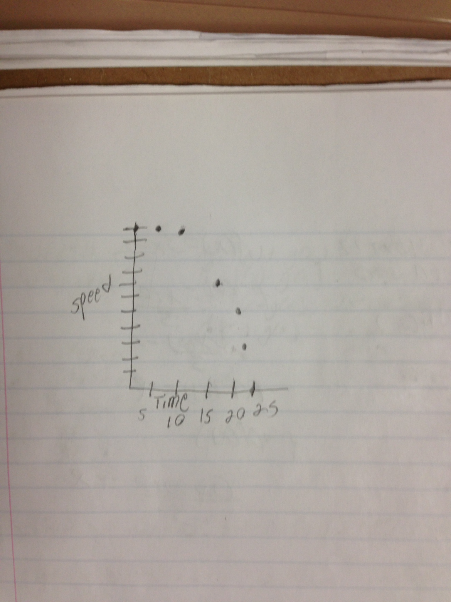
I ask the students to draw a graph of the speed of the car with respect to time. After playing the video a number of times, I had them share their graphs with their seat partner. As I circulated the room, I noticed their results fell into one of these three categories:
Graph A
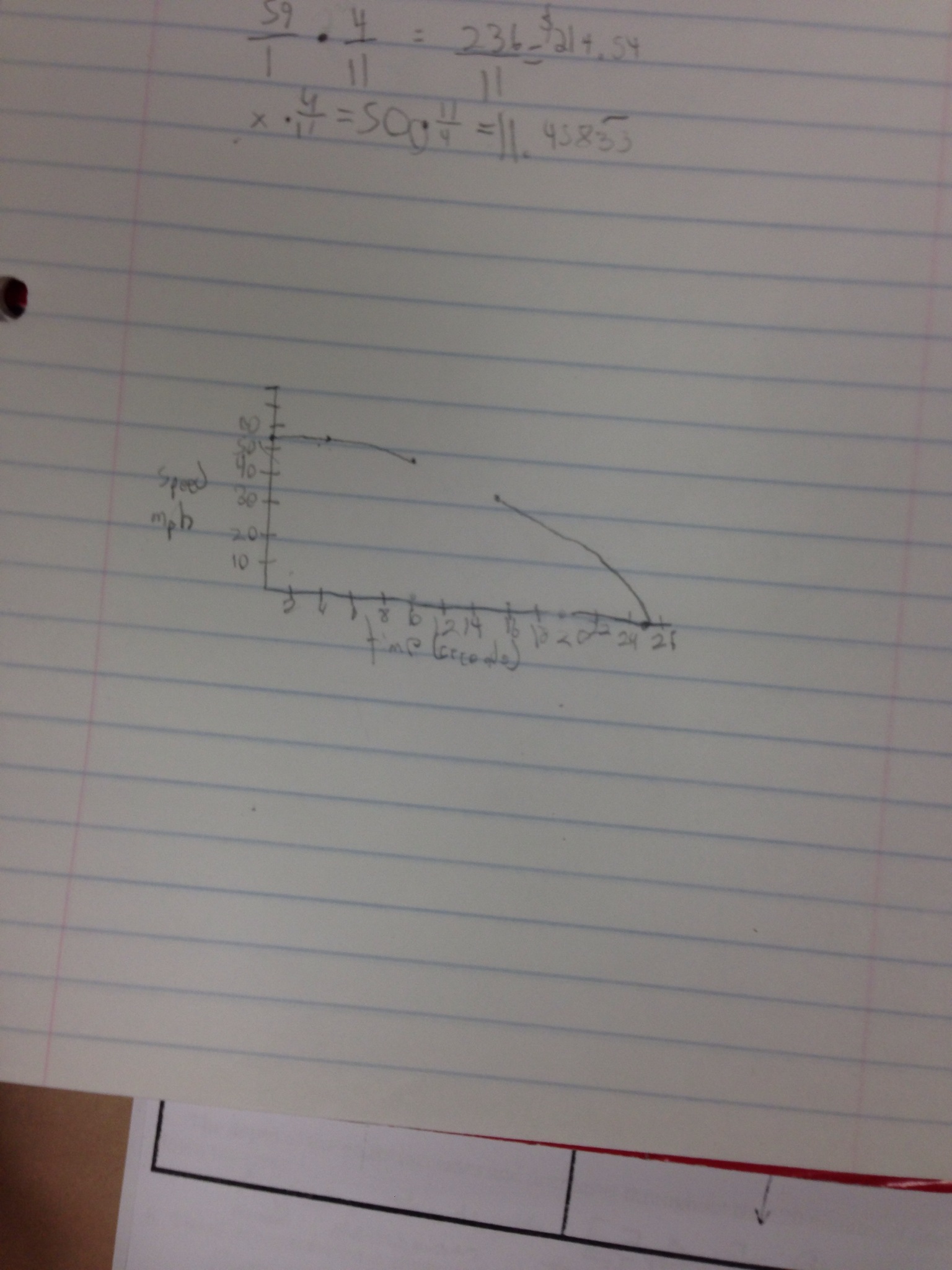
Graph B
Graph C
After examining the options, I had them choose which graph they felt represented the situation most accurately. Spoiler Alert: The overwhelming majority of them chose Graph B. Their reasoning: it’s unclear what happened to the speed between seconds 10 and 15 therefore, there should be a space in the graph. Those vying for Graph C cleverly argued that there was no audible “revving of the engine,” indicating that the car continued to slow. Others supporting C claimed that even though we could not see the speed, they know how a speedometer works and can make a reasonable assumption about what happened in that time frame.
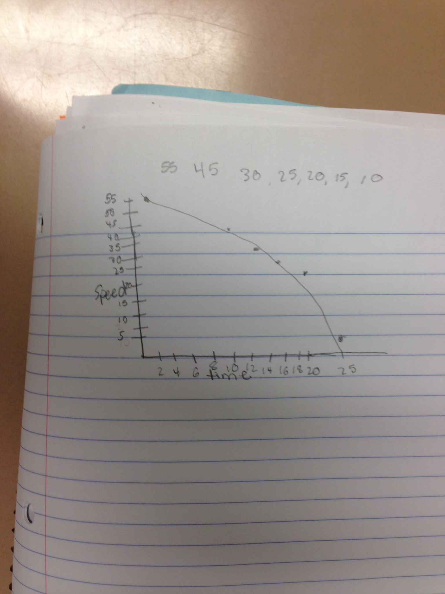
Enter this student’s graph and the Intermediate Value Theorem (trumpets):
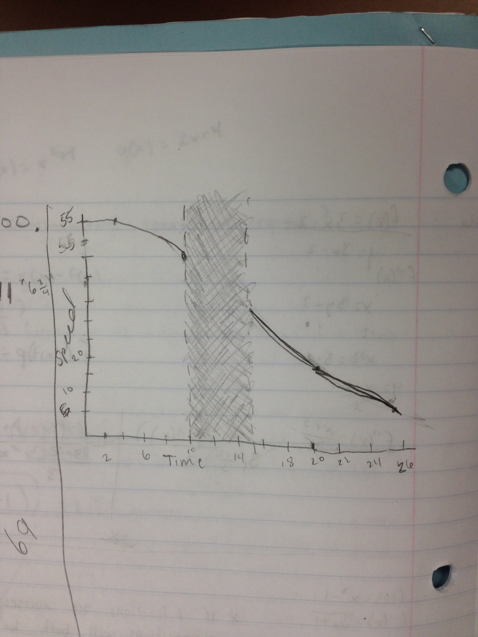
I liked this students “shading” through unknown speed region, so I projected it for everyone to discuss. They were able to determine the value of the function at ten seconds, f(10), was approximately 45 miles per hour and the value of the function at fifteen seconds, f(15), was approximately 35 miles per hour. They also knew that the car must have reached 40 miles per hour sometime in between 10 and 15 seconds. “How do you know that?” I pryed. Gem response of the day: “Well, speed is continuous and I can’t go from 45 mph to 35 mph without going through 44, 43, 42, 41, 40 mph, and so on.” Bingo. Intermediate Value Theorem. No boring procedural explanation necessary.
We applied this “new” knowledge to a polynomial function so that they could get a handle on some of the algebra and notation used. And as a bonus, they also seemed to grasp that this theorem does not only apply to crossing the x-axis, a common misconception students had last trimester.
Moving forward, I’ll definitely work on creating a better video!